| Introduction: |
| This applet calculates the property
variations across a normal or oblique shockwave under two
sets of assumptions. The first choice is the standard
assumption of a calorically (and thermally) perfect gas.
The gas can be any that meets the assumptions provided
The gas constant and specific heat ratio are known. The
second option is for standard equilibrium air at
densities from 1,000 amagats to 1e-7 amagats and
temperatures up to 25,000 K. This analysis accounts for
real gas effects of a standard mixture of species in air
including dissociation and ionization. This analysis is
generally quite accurate for values within the stated
density range, but can only be used with air. The program
provides many options for specifying upstream properties
and provides quick calculation. The output can be
summarized to be copied and pasted into a word processor,
and the applet provides a platform-independent,
easy-to-use interface. |
| Acknowledgements: |
| I would like to thank Dr. William Devenport and Dr. Bernard Grossman, as they are the
people who have written a very important part of this
code. Although the shock algorithms and interfacing have
been coded by me, the real gas effects algorithm
has been coded by them, with the original coding work
done by Dr. Grossman in FORTRAN. The curve fit
tables for this algorithm comes from [1]. The source code for this file
is quite complex, so I would like to thank them for
something which would be very difficult to reproduce!
More of their similar work can be found at www.engapplets.vt.edu. |
| Typical Steps for Solution: |
- Select the shocktype, either normal or oblique,
and under either real or calorically perfect
assumptions.
- Select units as convenient.
- Specify exactly 2 known upstream properties by
typing their values into the upstream boxes, and
select those two by selecting the checkboxes
appropriate to each. If the analysis is
calorically perfect, the user has the option of
entering no upstream properties instead, but, in
this case, the downstream ratios button is
automatically selected.
- If the analysis is of an oblique shockwave, enter
an angle in the appropriate box and select that
angle by checking the checkbox. For a calorically
perfect oblique shock, either theta or beta can
be entered. For a real oblique shock, only theta
is accepted.
- If the analysis is calorically perfect, make sure
that R and gamma are correct, or change their
values to fit the gas being analyzed.
- Enter either an upstream mach number or upstream
velocity and select the checkbox next to it.
- decide if either the ratios of downstream to
upstream or the downstream stagnation values are
desired and check those boxes as appropriate.
- That's it!! Hit the "Calculate" button
for the solution in the right hand column!
|
| Users Guide: |
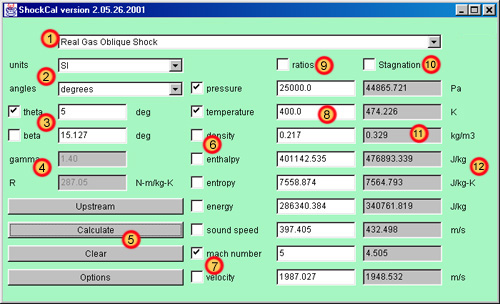 |
- Shock
Type Selection Choice - This
menu allows the uer to choose from four
different types of shockwaves. For the
assumptions and applicability of each
type of shockwave, see the technical theory
section below.
- Units
Choice - Choices are provided
for property units in either SI or
British systems of measurement and angles
in either degrees or radians. The boxes
of property and angle values are
succeeded by the specific appropriate
units, which will change depending on the
choices made here. Of course, make sure
that all values given to the program are
given in the units asked for.
- Angle
Specification - the angle
specification is used only for oblique
shocks (both calorically perfect and
real). Selecting a normal shock will gray
out this area. Most typically, theta is
known, but one of the two angles must be
known and specified to carry out this
analysis. Note that the real gas oblique
shock can ONLY accept theta as an input
parameter (it is unlikely that beta would
be known anyway). The calorically perfect
oblique shock accepts either. Indicate
which is the known quantity by checking
the appropriate checkbox. The other angle
that is calculated in the analysis is
filled in by the program as part of the
solution.
- Constants
Specification - The specific
heat ratio and gas constant are used only
for the calorically perfect shocks.
Selecting a real shock will gray out this
area. The default values are appropriate
for standard air at modest temperatures.
These parameters must be specified for
other gases. (see the technical
theory section below for information
on how to get these numbers for other
cases).
- Action
Buttons - Four buttons are
present which controls the actions of the
program.
- Upstream:
This button calculates
all upstream properties
for either a real or
calorically perfect gas.
Two properties must be
specified by the user in
order to calculate the
rest. Acceptable choice
of the two specified
properties are defined in
the technical
theory. If a mach
number or velocity is
specified, the code will
also calculate the other
upstream value.
Otherwise, this is left
blank. Entering invalid
data will generate an
error message.
- Calculate:
This button causes all
upstream data to be
calculated as in the
button above. Then, the
changes across the
shockwave are calculated
and displayed. If a real
gas shockwave, two
upstream properties, and
either mach or velocity
must be specified. If a
calorically perfect gas
shockwave, the same is
true, except that only
upstream mach number can
be specified if desired
(output is automatically
only the property ratios
however). Also, gamma and
R must be given in this
case. If the analysis is
an oblique shockwave, an
angle must also be given.
- Clear:
This button clears
all enteered data and
resets the screen for a
new analysis.
- Options:
This button brings up a
dialog box giving some
options for the program.
These options include how
many significant digits to
output (internally, all
values are double
precision), and the
option of showing a
results summary window of
each shock which a user
can copy and paste to a
text editor.

|
- Upstream
Property Selection - The
checkboxes are for letting the program
know which two thermodynamic quantities
the user has specified. The code will
read these two, and calculate the rest
when the Upstream or Calculate buttons
are pressed. The code requires exactly
two (and bars a user from entering more).
Not entering a valid number generates an
error message. For calorically perfect
shocks, no properties can be entered, but
this forces the code to generate property
ratios only. The technical
theory section lists acceptable
property choices for all types of shocks.
- Speed
Selection - For calculating
the changes across the shock, either
velocity or mach number must be specified
upstream. Mach number must be specified
for the calorically perfect shock with no
upstream properties. The checkbox
indicates to the code which is specified.
Not checking one box or not entering a
valid number next to the checked item
results in an error.
- Upstream
Properties/Speeds - These are
the fields for entering the upstream
properties. Of course, valid numbers must
be entered. Entering data in a box that
is not checked will be ignored by the
program, and exactly 2 properties and one
speed must be given for calculation. The
code fills in the rest of the values.
- Ratio
Checkbox - This option tells
the program to output the ratio of
DownStr./UpStr. instead of the actual
downstream values. Very often, the ratios
of downstream to upstream are more
informative than the actual values. This
can be combined with the Stagnation
checkbox (below).
- Stagnation
Checkbox - This option tells
the program to output the value of the
stagnation properties rather than static
values. Stagnation properties are
described in the technical
theory section. This can be combined
with the ratio checkbox to ouput the
ratio of downstrean stagnation properties
to upstream stagnation value(i.e.
Po2/Po1, To2/To1, etc.).
- Downstream
Properties/Speeds - These are
the fields in which the results of the
calculations are displayed. They are not
editable (although the are copyable).
Selecting the ratios checkbox makes them
the ratio of downstream to upstream
properties. Selecting the stagnation
checkbox gives the stagnation properties
downstream.
- Units
- These are the units of the properties,
which are updated depending on the choice
of units. These units apply to both
upstream and downstream, unless the
ratios checkbox is selected, in which
case, downstream ratios are
dimensionless.
|
|
| Technical Theory: |
Only a brief technical
theory highlighting important points is presented here.
Most of the theory used in this applet is documented in
well-established sources,
complete with derivations and equations.
First, the difference between a real and a calorically
perfect gas is discussed. A calorically perfect gas is
one in which the specific heats of the gas are constant.
This is the relationship between the amount of energy in
a gas to its temperature. A calorically perfect gas is
one in which the specific heats do not vary as
temperature increases or decreases. This is usually a
good assumption for diatomic gases at moderate
temperatures (around room temperature, or 300K). At
significantly higher temperatures, the gas tends to
dissociate and eventually ionize. Monatomic gases behave
similarly, except that they can't dissociate, so
calorically perfect validity tend to hold to much higher
temperatures. If unsure, a good way to get a
"feel" for the validity of the calorically
perfect assumption is to try both real and calorically
perfect normal shocks and compare answers. By raising the
upstream mach number in increments, an analyst will see
that at low mach numbers, both methods give similar
downstream temperatures. As mach number increases, one
will see that the calorically perfect assumption begins
to predict temperatures much higher than for the real
gas. This discrepency continues to grow with mach number.
The real gas effects are modeled by curve fit equations
from [1] as coded by Dr.
Grossman and Dr. Devenport(see above).
These curve fits are quite involved and a reader is
referred to that paper for more information on the
details of the fits. The equations are valid for 1,000 to
1e-7 amagats and less than 25,000 K.
For the calorically perfect gas, the gas constant(R) and
specific heat ratio(gamma) must always be specified. For
air, the correct values are 1.40 for gamma, and 287.05
J/kg-K or 1716.20 lbf-ft/slug-R for R. These two numbers
can be easily found for other gases as follows(from [3]): for any calorically perfect
gas, gamma can be assumed to be 7/5 for any diatomic gas,
and 5/3 for any monatomic gas. Also, R can be found by
taking the universal gas constant, 8314 J/kgmol-K, and
dividing by the molecular weight of the gas in question.
The calorically perfect formulation is the standard
formulation given in many compressible flow books. [2] is a particularly good book
and is recommended to learn the mechanics of this
program. The calorically perfect shockwaves are solved
exactly as outlined in chapters 3 and 4. Normal shocks
are solved directly using the formulas for pressure,
temperature, and density ratios given in chapter 3, which
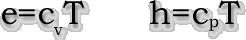
are functions only of mach number and gamma. Energy and
enthalpy are obtained by the calorically perfect
assumptions
|
 |
| Also, there is no analytical solution
given for the absolute value of entropy given for a
calorically perfect gas, except if based on a reference
point. The label for entropy changes to "entropy
change" for a calorically perfect analysis, and the
upstream value is set to the reference value. The
downstream solution is actually the entropy change, as
given: |
 |
For the oblique shock, first the
derivative of the famous beta-theta-mach equation (see [2], chapter 4) is solved to find
the maximum allowed theta, and corresponding beta are
found. If the input theta is greater than theta_max, the
shock is detached rather than oblique. This forms a
complex flow field beyond the abilities of this program.
Near the detachment point, a detached shock is more
closely represented by a normal shock. Provided theta is
less than theta_max, the beta-theta-mach equation is
solved using the bisection method, and the normal
upstream and downstream values are found as shown in [2].
For the real gas solutions, most of the algorithms are
iterative, solving the general jump conditions for a
normal and oblique discontinuity by the bisection method [3]. This makes the solution of
real gas equations more complicated and less reliable.
For the oblique shock, only theta is allowed as an input,
and since there is no analytical solution like the
beta-theta-mach relation, the code runs a calorically
perfect solution first to estimate whether theta exceeds
theta_max. If this happens, the program will simply give
erratic results and a warning is displayed. Also, through
the iterative process, if the algorithm detects a point
out of range of the real gas curve fits, it prompts the
user with a warning. [4] and [5] give a great deal of
background information on the handling and effects of
real gases.
A stagnation property is defined as "what the value
would be if the fluid was brought isentropically to a
halt under the current circumstances." For
stagnation properties in the calorically perfect case,
the stagnation pressure, temperature, and densities are
again calculated from the formulas of [2]. Stagnation enthalpy and
energy ratios are equal to the stagnation temperature
ratio. Note that the stagnation temperature ratio is
actually calculated even though it should always be 1.
This is done as a check on the program. For both real and
calorically perfect gases, by definition, static and
stagnation entropy is identical!
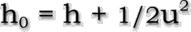
For real gases, the stagnation enthalpy is calculated by
definition from the jump conditions of a general fluid as
follows: |
 |
and the attribute that stagnation
properties are defined isentropically. Using the
calculated stagnation enthalpy, and entropy from the
solution, the real gas algorithm calculates the rest of
the properties. By definition in both cases, velocity is
zero.
The program (except under the ratio option of calorically
perfect gases) requires exactly 2 upstream properties and
and upstream mach number or speed to calculate -- plus
and angle for oblique shocks. For the calorically perfect
gas, acceptable parameter pairs are: |
| pressure |
temperature |
| pressure |
density |
| temperature |
density |
| density |
enthalpy |
| density |
energy |
| pressure |
enthalpy |
| pressure |
energy |
|
| For the real gas air tables, acceptable
property pairs are as follows: |
| pressure |
temperature |
| pressure |
density |
| density |
energy |
| entropy |
enthalpy |
| pressure |
entropy |
|
| Tips for Use: |
- because of the extreme narrowness of the
solution, the iterative algorithm for the real
oblique shock doesn't work well for M1 less than
1.5 or so. For 1 < M1 <1.75 or so, use the
calorically perfect oblique shock instead. It is
capable of solving down virtually to M1 = 1, and
low mach numbers are the cases when the
calorically perfect assumptions hold the best.
- for a real oblique shock, the beta-theta-mach
equation is solved for a calorically perfect case
in order to determine if the maximum theta has
been exceeded and the shock is detached. If this
happens, the real oblique shock will still
provide whatever is gets, but a warning is
displayed, and the solution is probably not valid
at all.
- when in doubt, try a shock solution as both real
and calorically perfect, and compare answers. In
general, the higher the incoming mach number, the
larger the discrepency.
- MAKE SURE THE UNITS MATCH WHAT THE PROGRAM IS
ASKING FOR(Including RADIANS vs. DEGREES)!!!
- across all non-moving shocks, the stagnation
enthalpy should remain the same. Therefore,
selecting "ratios" and
"stagnation", the downstream enthalpy
reading should be very close to 1 (within a
little numerical rounding). The same is true for
stagnation temperature for calorically perfect
gases. This is a good check that the program
executed correctly.
|
| References: |
| [1] |
Srinivasan S, Tannehill J C and
Weilmuenster K J. "Simplified Curve Fits for the
Thermodynamic Properties of Equilibrium Air", NASA
RP1181, August 1987. |
| [2] |
Anderson, John. Modern Compressible
Flow. 2nd ed. ISBN#0-07-001673-9. McGraw-Hill, 1990. |
| [3] |
Grossman, Bernard. "Fundamental
Concepts of Real Gasdynamics". Virginia Tech/AOE
department. Class notes, AOE5114, High Speed
Aerodynamics. Version 3.09, January 2000. |
| [4] |
Vincenti, W.G. and Kruger, C.H. Introduction
to Physical Gas Dynamics. New York: Wiley,1965. |
| [5] |
Liepmann, H.W. and Roshko, A. Elements
of Real Gasdynamics. New York: Wiley, 1957. |